|
|
TX to Ae | RF Bridges | - | - |
6.4 Reflectometry
(Measurement of reflection coefficient, return loss, and SWR)
>>> work in progress.
Reflectometry:
One of the principal applications of the impedance bridge is the measurement of forward and reflected power in transmission lines; this usually being expressed in terms of SWR or return loss (to be defined shortly). The bridge however, cannot measure reflections, it can only measure quantities which can be derived from voltage and current. The ratio of forward to reflected power in a line is a function of the load impedance and the characteristic impedance; and, in the case of a lossless line at least, remains constant throughout the length of the line. The actual input impedance of a mis-terminated line however, can vary radically depending on its length; and so impedance on its own is not sufficient to determine the required power ratio. The key to reflectometry therefore, is to devise bridges which can measure some quantity which is conserved regardless of the length of the line, and to derive the required information from that.
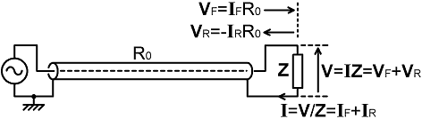
Consider a wave traveling from generator to load in a lossless transmission line. As the wave moves along the line, it has no knowledge of the conditions it will meet when it arrives at the load; and so the relationship between voltage and current in the forward traveling wave is dictated entirely by the surge resistance (i.e., the characteristic resistance), R0, of the line. Thus we may write:
| VF = IF R0 |
( |
If the line is not terminated in its characteristic resistance, only part of the energy in the wave will be absorbed (or perhaps none if the line is open or short-circuit), and a reflected wave will be launched on a journey from the load to the generator. This reflected wave will also have no knowledge of the conditions which prevail at its destination, and so the relationship between voltage and current will also be determined solely by R0, i.e.,
| VR = -IR R0 |
|
In this case, a minus sign is required in order to maintain consistency in the definitions of the forward and reflected waves; i.e., we must assume that either the voltage or the current is reversed relative to the forward wave at the reflection boundary. To understand this point, note that if the line is open circuit, a voltage may exist at the discontinuity, but the sum of forward and reflected currents must be zero, i.e., the sign of the current must reverse as the wave turns around and heads back towards the generator. Conversely, if the line is short circuit, then a finite current may exist at the end of the line, but the sum of the forward and reflected voltages must be zero, i.e., the sign of the voltage must reverse. When partial reflection occurs, the voltage reverses relative to the forward wave if the magnitude of the load impedance is less than R0, and the current reverses if the magnitude of the load impedance is greater than R0; but the minus sign in the expression above maintains consistency in either case, and allows the forward and reverse wave definitions to be combined (i.e., to be used as simultaneous equations).
We cannot, of course, measure the forward and reflected voltages and currents independently. If we make measurements of voltage and current at various points on the line, we will always measure the sum of forward and reflected voltages and the sum of forward and reflected currents at each point. At the load however, we can determine the relative magnitudes of the forward and reflected voltages or currents, because the relationship between the total voltage and the total current at this point is defined by the load impedance Z. The ratio so determined is called the reflection coefficient, and is true of the magnitudes of the forward and reflected voltages and currents at any point in the line because the power (energy per unit of time) in the forward and reflected traveling waves is constant. An expression for the reflection coefficient can be determined as follows:
If V is the voltage across the load, and I is the current flowing through the load, then we may write:
| V = I Z = VF + VR . . . (3) |
| I = V / Z = IF + IR . . . (4) |
The observations made so far are summarised in the diagram below:
From the relationships given above, we have IF=VF/R0 and IR=-VR/R0. Substituting these expressions into equation (4) gives:
I = (VF / R0) - (VR / R0) = (VF - VR) / R0
and using (3) gives:
(VF + VR) / Z = (VF - VR) / R0
which can be rearranged as follows:
(VF + VR) R0 = (VF - VR) Z
VF R0 + VR R0 = VF Z - VR Z
VR R0 + VR Z = VF Z - VF R0
VR (Z + R0) = VF (Z - R0)
To give:
| VR / VF = (Z - R0) / (Z + R0) |
| |VR| / |VF| = |Z - R0| / |Z + R0| |
The quantity |VR|/|VF| is the desired reflection coefficient, and is variously given the symbol ρ (rho), Γ (capital Gamma), or k, depending on the commentator. Here we will prefer Γ, because ρ is already used elsewhere to denote both resistivity and density. Γ is sometimes called the "voltage reflection coefficient", but this is a peculiar affectation as we may see by using relationships (1) and (2) to eliminate all voltages from equation (3); and then using equation (4) to eliminate I. By so doing we obtain:
IF Z + IR Z = IF R0 - IR R0
which rearranges to:
| -IR / IF = (Z - R0) / (Z + R0) |
| |IR| / |IF| = |Z - R0| / |Z + R0| |
Thus, to summarise:
|
Γ = |
|VF| |
|
|IF| |
|
| Z + R0 | |
>>> work in progress
Lossy lines:
Z0 = R0 + jX0 (X0 is negative) and Z0*
Return loss = 20Log10( 1/Γ ) [dB]
SWR
S=Max peak voltage/min peak voltage = Max peak current/min peak current
(Only strictly defined for lines of λ/4 and longer)
S = ( 1+Γ ) / ( 1-Γ )
True for any length of line and for lossy lines.
Γ = (S-1)/(S+1)
Γ = √(PR/PF)
>>>
Directional coupler:
The transmission line between a radio transmitter and an antenna does not necessarily need to be matched; but the presence of standing waves on an unmatched line creates a problem of power measurement when the intrumentation (as is usually desirable) is located in the radio room. The line performs an impedance transformation such that, at a distance of λ/4 (an electrical quarter-wavelength, or 90 electrical degrees) from the load, the impedance looking into the line will be of high magnitude if the magnitude of the load impedance is less than the characteristic resistance of the line, and vice versa. The impedance varies cyclically as the distance from the load increases, and returns to the same value (neglecting losses) at intervals of λ/2. Since the length of the line is usually dictated by the physical installation rather than by electrical considerations; early attempts to monitor transmitter performance by measuring either the voltage or the current at the transmitter terminals were bound to produce inconsistent results.
>>
Invention of: (early patents). Overcoming misleading measurements by taking average of voltage and current analogs at a given point.
Gothe, Buschbeck, Kautter 1939, US 2165848 .
Alexander 1949 US 2467648 .
the directional coupler is related to the telephone hybrid circuit, a device used for separating and recombining upstream and downstream signals in long telephone lines so that the separated signals can be passed through amplifiers. Also used to reduce side tone, so that callers are not deafened by their own voices. The name 'hybrid' probably derives from the fact that any particular transformer winding is neither a primary or a secondary, but performs both functions simultaneously.
Determining Γ as an analog computation problem.
|
Γ = |
|VF| |
|
|IF| |
|
| Z + R0 | |
|
| Vv + Vi | |
>>>>> to be rewritten
6.4-x. The Reflectometer (or SWR) bridge:
An SWR bridge is a reflectometer bridge with a meter scale calibrated in SWR. A reflectometer bridge is a set of two impedance bridges; one used normally, and one used with the generator and the load transposed.
When an impedance bridge is designed to balance at the characteristic resistance (R0) of a transmission line into which it is inserted, the balance condition, by definition, occurs when the power reflected back from the load is zero; i.e., the bridge indicates whether or not the transmission line is correctly terminated, and it transpires that any imbalance reading is proportional to the square-root of the reflected power. If the load and the generator are transposed however, the bridge will no longer balance, because the output at the detector port is now Vv+Vi rather than Vv-Vi (the polarity of the current sample is reversed). The configuration is still useful however, because it solves the problem of how to measure the forward power in a transmission line in the presence of standing waves. If there is reflected energy travelling in a line, the voltage on the line will be the sum of the voltages due to forward and reflected power, and this will vary sinusoidally with the distance from the load. Hence, if the forward power is to be measured at an arbitrary point on the line, it cannot be calculated from |V|²/R0. Similarly, the current in the line will vary sinusoidally, and the forward power cannot be calculated from |I|²R0. Current maxima however will always correspond to voltage minima, and vice versa, and so the forward power can be deduced by making two determinations, one from the current and one from the voltage, and taking the average. Hence |Vv+Vi| is proportional to the square root of the forward power, provided that the current and voltage samples are taken at exactly the same electrical point on the line.
In a current-transformer bridge with more than one turn in the current-transformer primary winding, an apparently sensible point at which to sample the voltage is at a primary centre tap. Since most bridges only have one primary turn however, the voltage must be taken from one side or the other, but the error which results is negligible provided that the distance from the middle of the current transformer is small in comparison to one wavelength at the highest frequency of operation. Such is the accepted practice, but in fact it is not always best to sample voltage and current at exactly the same physical point; because it takes time for the current sample to propagate out of the transformer coil. The best technique is to take voltage and current samples from points of equal time-delay ralative to the source, a matter which can be dealt with by neutralisation, or by moving the sampling point down-line by an electrical distance equal to half the electrical length of the current-transformer secondary winding.
A prototype SWR bridge is shown below: where the magnitude of Vf is proportional to the square-root of the forward power and is independent of reflected power; and the magnitude of Vr is proportional to the square-root of the reflected power, and is independent of forward power.
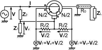
Since the output of the current transformer is shared between two bridges, the balance condition is now:
Vv - Vi/2 = 0
This means that the voltage sampling network components must be chosen to give half the output required for a single bridge, but the bridge design procedure is otherwise the same.
Caveat: Notice that the dual bridge circuit shown above has a serious flaw in one of its most popular implementations; which is that in which the voltage sampling network Z1, Z2 is a high-impedance capacitive potential divider, the forward and reflected output ports are terminated with diode detectors, and the circuit is used to drive two meters simultaneously. When the load ZL is correctly matched to the cable, the forward output will be large and will drive its detector hard; causing the output of the voltage sampling network to droop, especially at low frequencies. This will throw the balance condition for the reflected power bridge and give rise to a spurious reading. Essentially, the shared capacitive-divider version does not work properly at low frequencies when used to drive two separate meters, it being an ill-conceived extension of a circuit intended to have a single meter and a switch to select between forward and reverse readings. Warren Bruene's solution to this problem was to use separate voltage sampling networks for the two bridges [40]. Also, if we decide to compensate for current-transformer delay by moving the voltage sampling point along the line, we will need to move the reflected power voltage network towards the load and the forward power voltage network towards the generator, and so we will be forced to use two voltage sampling networks anyway. Another solutions are to use a voltage sampling network with a low output impedance.
It was mentioned in the last paragraph, that in order to delay the voltage sample for reflected power, it is necessary to move the sampling point towards the load. This might seem anti-intuitive, but only if we subscribe to the view that the reflectometer can measure reflected power. It can do no such thing: it can only infer the existence of reflected power from the difference between the actual load impedance and the target load impedance. To understand this point, consider an SWR bridge designed to balance when the load is 50+j0Ω. If we connect this bridge directly to a 100Ω load resistor, it will declare an SWR of 2:1. The resistor is not reactive however, and so will absorb all of the power delivered to it and reflect none. The 2:1 SWR reading is only true when the bridge sees an impedance magnitude of 100Ω (or 25Ω) at the input to a 50Ω transmission line. The bridge is just an impedance bridge, it has no special psychic powers, and its readings are only true when it is inserted into a line having the same characteristic resistance.
6.4-x. The Bruene Directional Wattmeter:
>>> To be rewritten.
>>>> The Bruene bridge is discussed below because it is historically interesting. It is not recommended as a basis for modern designs.
The "Directional Wattmeter" (i.e., SWR bridge) circuit shown below is based on a circuit devised by Warren Bruene (W0TTK, W5OLY, of the Collins Radio Company) which became popular among radio amateurs as a result of an article published in 1959 [40]. The original Bruene bridge was essentially the same as Douma's bridge, but without low-frequency compensation and rearranged to use the shunt-diode detector configuration [see Detectors for RF meas.]. These changes were sufficient to circumvent Douma's 1957 patent [USP 2808566], but the circuit is also a logical development of the capacitor ratio-arm bridge (CRAB) used in earlier Collins designs and so may well have been invented independently. The CRAB used as a mismatch (SWR) indicator in the Collins 180L-3 (2 MHz - 25 MHz) automatic antenna tuner is discussed elsewhere [ /zdocs/zmatching/ ]. A "high-frequency iron" toroidal current transformer was however used for the phase and magnitude bridges of that unit, and so it was only a matter of time before the toroid migrated into the reflectometer. The CRAB was used down to 2 MHz however (limited only by the output impedance of the ratio arms); whereas the lack of LF compensation in the original Bruene bridge raised the useful minimum frequency, and the designs discussed in references [40], [41], and [42] are only suitable for 3.5-30 MHz. Douma's patent expired in 1977, and so, while home constructors never had valid reason to omit the compensation resistors (apart from lack of awareness of their importance), commercial designers now have no reason to omit them either (and probably never did, because Douma did not invent this compensation method - it was used by Korman in 1942 [US Pat. 2285211] and so was out-of-Patent by 1962). Consequently, the resistors (Rv) have been added to the circuit shown below, and their inclusion should be regarded as mandatory. The inclusion of compensation resistors also necessitates the inclusion of blocking capacitors (Cb) to prevent the DC outputs of the detectors from being shunted to ground. Cb merely needs to have a low reactance at the minimum frequency of operation (10 nF ceramic will usually do the trick) but an excessively large capacitor (i.e., several μF) in this position will slow the rate at which the DC output can change and will damp the meter response.
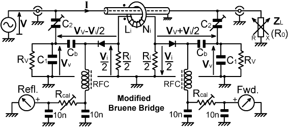
Notice that the shunt-diode detector is connected directly between the current and voltage sample outputs and the rectified signal is extracted through an RF choke (RFC). This floating detector configuration is a Hallmark of the Collins Radio Company from the 1950s; but is perhaps nowadays somewhat archaic. One disadvantage is that the detector 'ports' are not referenced to ground, and so isolation transformers will be required if signals are to be injected into them. Note also that the RF chokes must be carefully chosen to have a very high impedance throughout the operation frequency range, since reactive loading of the voltage sampling network will introduce serious errors into the balance condition (multi-segment RF chokes of 1mH or more are normally used). If the drop in meter sensitivity which results from using Rv as the detector DC return path can be tolerated, it is a good idea to swap the detector connections, i.e., connect the anode of the diode to the junction of C1 and C2, and connect the blocking capacitor Cb to the current transformer output. Due to the very low output impedance of the current transformer circuit, self-capacitance effects in the choke will then only affect the magnitude of the meter reading and will have little effect on the balance condition. If the detector is reversed in this way incidentally, attempting to restore its sensitivity by connecting a choke across Rv is not a good idea; but as we shall see by performing an actual design calculation, the loss of sensitivity will not be particularly large because Rv will be measured in hundreds rather than thousands of ohms.
The balance condition is:
Vv - Vi/2 = 0
where, from the derivation given in section ?:
Vv/V = ηv = (Rv // jXC1 // jXC2) / jXC2
and the current transfer function at balance (from section ?) is:
Vi/V = η0 = (jXLi // Ri) / Ni R0
Since the current sample is shared by two bridges, we must divide it by two. Hence, at balance:
ηv = η0/2
i.e.,
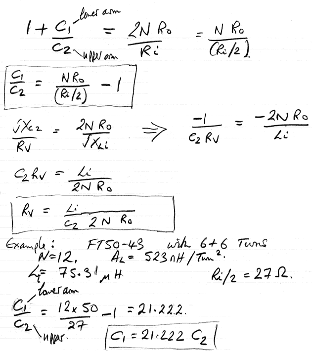
(Rv // jXC1 // jXC2) / jXC2 = (jXLi // Ri) / (2 Ni R0)
which upon inversion of both sides gives:
jXC2 [(1/jXC1) + (1/jXC2) + (1/Rv)] = 2Ni R0 [(1/Ri) + (1/jXLi)]
Recalling that XC=-1/2πfC and 1/j=-j, this rearranges to:
[(C1+C2)/C2] + jXC2/Rv = [2Ni R0 / Ri] - j2Ni R0/XLi
Hence, equating the real parts:
| (C1+C2)/C2 = 2Ni R0/Ri |
|
and, equating the imaginary parts:
| 1/C2Rv = 2Ni R0/Li |
|
Example:
A Bruene bridge design is given in ref. [41]. This uses an Amidon T68-2 core with 35 turns of #26AWG enamelled wire, and the current transformer secondary load is 20 Ω, i.e., the two resistors marked Ri/2 above are 10 Ω each. The capacitors here designated C1 were originally 330 pF, and capacitors C2 were 7 pF trimmers. Low-frequency compensation resistors were not used in the original circuit, and the operating frequency range was stated to be 3.5 to 30 MHz; but since we have data for the transformer core we can compute values for the compensation resistors and extend the frequency range to 1.8 MHz.
Using equation (x.1) we will first find the nominal capacitance of C2 when the bridge is balanced for 50 Ω loads:
(C1/C2) + 1 = 2Ni R0 / Ri = 2×35×50/20 = 175
C1/C2 = 174
330 pF = 174C2
C2 = 1.90 pF
This has a reactance of -24 kΩ at 3.5 MHz and -46.6 kΩ at 1.8MHz. To stay roughly in keeping with the original design intentions we should increase C2 to obtain a reactance of about -24 kΩ at 1.8 MHz, and so a candidate value for C2 is 3.68 pF and C1=174C2=641 pF. 680 pF is the larger nearest preferred value, and 1% silvered-mica capacitors of this value are available, and so we end up with C1=680 pF, C2=680/174=3.9 pF (obtained by adjusting a 2-10pF trimmer). Since there are two voltage sampling networks, our choice will result in a fixed capacitance of nearly 8 pF across the generator, but since one of the networks is on the load side, it will be absorbed into the load impedance after adjustment. Hence the mismatch seen by the generator when the bridge is balanced will be mainly due to the presence of only one of the voltage sampling networks, and the effect of 3.9 pF is comfortably within normal load tolerance limits.
For low frequency compensation, we note that the transformer has 35 turns, and the AL value of the T68-2 core is 5.7 nH. Hence the secondary inductance is ALN²=7 μH. Using equation (x.2):
Rv = Li/2Ni R0C2 = 7×10⁻⁶ / ( 2 × 35 × 50 × 3.9×10-12 ) = 512 Ω
A measurement of the actual inductance of the transformer coil is, of course, a better criterion for the calculation of the compensation resistor.
In the matter of setting the balance points and calibrating such a bridge, notice that the circuit is completely symmetric. Having connected a 50 Ω resistor to the load port and adjusted the reflected-signal voltage-sampling network for a null reading on the corresponding meter, the generator and load connections can be swapped for adjustment of the other trimmer. For calibration of the meter scales, the voltage across the load can be measured (e.g., using a calibrated oscilloscope and a ×10 probe, provided that the 'scope input voltage rating is not exceeded), swapping the generator and load connections as before for adjustment of the two meter series resistors. For very high-power transmitters, the voltage should be measured at the output of a through-line attenuator (i.e., a tapped dummy-load resistor). Recall that forward power is proportional to the square root of Vv+Vi, and so the meters will have to be fitted with non-linear scales if calibrated in watts or relative power. It is quite common for the meter resistors to be switched for different FSD power readings. Dual-gang variable potentiometers are also used, but the tracking of inexpensive double potentiometers, particularly of the logarithmic variety, is notoriously bad. Since most transmitters have a drive-level control, infinite variability of the bridge sensitivity is not usually needed, and switched ranges calibrated in actual power are much more useful. Note that the accuracy of the calibration at low frequencies depends on the relationship between XLi and Ri as discussed in section ?. In the example given above XLi=4Ri at 1.8 MHz, and so the error will be less than 5% (see table ?); but in that case the design is for use in conjunction with kilowatt transmitters, and more sensitive designs (less turns on the current transformer core or a larger value of secondary load resistance) will not be so good in this respect.
>>>>>
Use of transformers to take off |Vv±Vi |. Gets rid of the chokes and costs about the same.
>>>>
Refs
[40] "An Inside Picture of Directional Wattmeters", Warren B Bruene W0TTK [W5OLY], QST April 1959 p24-28.
[41] "In-Line RF Power Metering" Doug DeMaw W1CER [W1FB], QST Dec 1969 p11- 16.
Construction article for Bruene-type bridges for 3.5-30MHz.
[42] Ferromagnetic Core Design & Application Handbook, M F "Doug" DeMaw W1FB, 1st edition, 2nd printing 1996. MFJ publishing co. http://www.mfjenterprises.com/ .
Bruene bridge: p94-95.
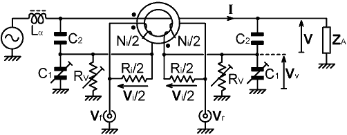
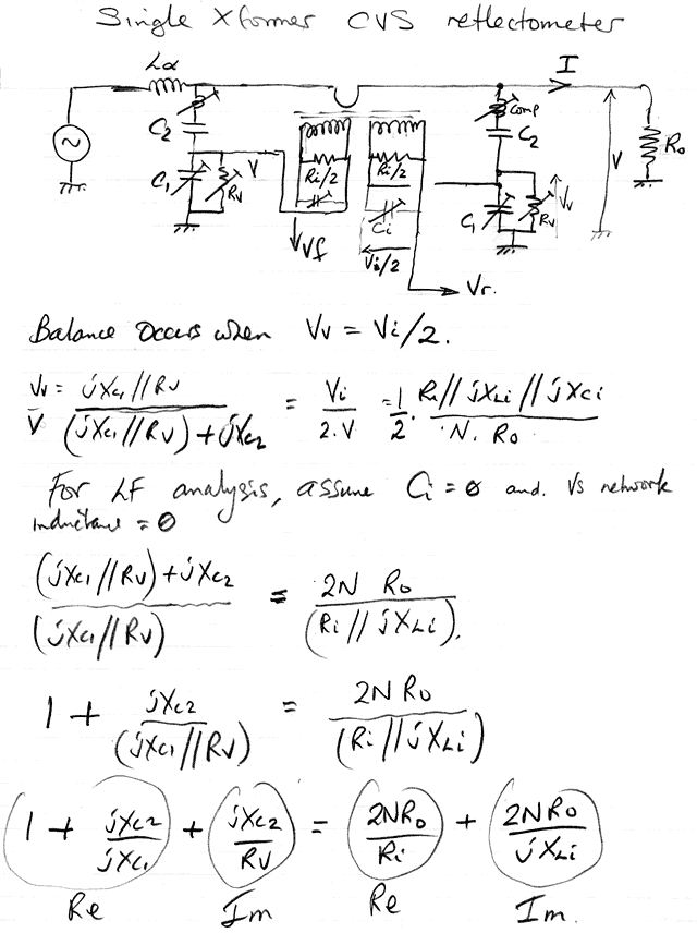
6.4-x. SWR Bridge with load-side voltage sampling.
>>>>>
Same basic design considerations as Bruene.
Inductance of half winding is Li /2 as explained in section 6-x.
Gets rid of the chokes.
Gets rid of the loading defect of shared voltage-sampling networks.
CVS network across load allows neutralisation by the load-capacitance method. HF phase neutralisation can be effected by arranging CVS network capacitance to be larger than required, then adding a small amount of capacitance across the transformer secondary.
HF amplitude correction (compensation for inductance of lower voltage-sampling arm) can be effected by placing a small inductance in series with C2.
Ground referenced det. ports allow reciprocal calibration and stealth tuning (must short Lα during the calibration reversal)
Lα calculated as per section 6-x, compensates for capacitance across the line.
Rv can be a resistor in series with small pot.
C1 can be a fixed capacitor in parallel with a trimmer.
Power Measurement
6.4-x. Square-Law detectors:
A section on the use of square-law detectors in power measurement.
Large signal "linear" detector.
Small signal. Output voltage is proportional to the square of the input voltage
Agilent application notes [see diode detectors].
The square root of a number can be obtained by halving its logarithm and taking the antilog.
Log and antilog amplifiers. Temp compensation using dual transistors.
>>
© D W Knight 2008, 2013.
David Knight asserts the right to be recognised as the author of this work.
Last edited:2021 Sept 12th (but still not conforming to HTML 5)
|
|
TX to Ae | RF Bridges | - | - |